Fold - Core Walkthrough

Welcome 👋
In this notebook we'll demonstrate fold's powerful interface for creating, training, and cross-validating (or backtesting, if you prefer) simple and composite models/pipelines.
We will use the dataset from an Energy residual load forcasting challenge hosted on Kaggle.
By the end you will know how to: - Create a simple and ensemble model (composite model) - Train multiple models / pipelines over time - Analyze the model's simulated past performance
Let's start by installing:
- fold
- fold-wrappers: optional, this will be required later for third party models. Wraps eg. XGBoost or StatsForecast models to be used with fold.
- krisi, optional. Dream Faster's Time-Series evaluation library to quickly get results.
Installing libraries
%%capture
pip install --quiet fold-core fold-wrappers fold-models krisi matplotlib seaborn xgboost plotly prophet statsforecast statsmodels ray kaleido
Data Loading and Exploration
Let's load in the data and do minimal exploration of the structure of the data.
fold has a useful utility function that loads example data from our datasets GitHub repo.
- We are forecasting
residual_load‡. - We will shorten the dataset to
4000rows so we have a speedier demonstration.
‡ The difference between the load in the network and the P that the industrial complex is producing.
from fold.utils.dataset import get_preprocessed_dataset
from statsmodels.graphics.tsaplots import plot_acf
from krisi import score, compare
from krisi.report import plot_y_predictions
import plotly.io as pio
pio.renderers.default = "png"

X, y = get_preprocessed_dataset(
    "energy/industrial_pv_load",
    target_col="residual_load",
    resample="H",
    deduplication_strategy="first",
    shorten=4000,
)
no_of_observation_per_day = 24
no_of_observation_per_week = no_of_observation_per_day * 7

y.plot(figsize = (20,5), grid=True);
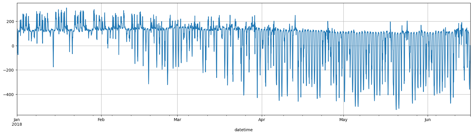
The data format may be very familiar - it looks like the standard scikit-learn data.
X represents exogenous variables in fold, where a single row corresponds to a single target value. That means we currently only support univariate time-series (with exogenous variables), but soon we're extending that.
It's important that the data should be sorted and its integrity (no missing values, no duplicate indicies) should be checked before passing data to fold.
| P | Gb(i) | Gd(i) | H_sun | T2m | WS10m | load | residual_load | |
|---|---|---|---|---|---|---|---|---|
| datetime | ||||||||
| 2018-01-01 00:00:00 | 0.0 | 0.0 | 0.0 | 0.0 | 8.44 | 5.54 | 120.0 | 120.0 |
| 2018-01-01 01:00:00 | 0.0 | 0.0 | 0.0 | 0.0 | 7.56 | 5.43 | 115.5 | 115.5 |
| 2018-01-01 02:00:00 | 0.0 | 0.0 | 0.0 | 0.0 | 7.04 | 5.33 | 120.5 | 120.5 |
| 2018-01-01 03:00:00 | 0.0 | 0.0 | 0.0 | 0.0 | 6.48 | 5.67 | 123.5 | 123.5 |
| 2018-01-01 04:00:00 | 0.0 | 0.0 | 0.0 | 0.0 | 5.95 | 5.79 | 136.5 | 136.5 |
(We'll ignore the exogenous variables until a bit later)
datetime
2018-01-01 00:00:00    115.5
2018-01-01 01:00:00    120.5
2018-01-01 02:00:00    123.5
2018-01-01 03:00:00    136.5
2018-01-01 04:00:00    138.0
Freq: H, Name: residual_load, dtype: float64
You can see that y (our target) contains the next value of X's "residual_load" column.
Time Series Cross Validation with a univariate forecaster
1. Model Building
fold has three core type of building blocks which you can build arbitrary sophisticated pipelines from:
- Transformations (classes that change, augment the data. eg: AddHolidayFeatures adds a column feature of holidays/weekends to your exogenous variables)
- Models (eg.: Sklearn, Baseline Models, third-party adapters from fold-wrappers, like Statsmodels)
- Composites (eg.: Ensemble - takes the mean of the output of arbitrary number of 'parallel' models or pipelines)
Let's use Facebook's popular Prophet library, and create in instance.
If fold-wrappers is installed, fold can take this instance without any additional wrapper class.
2. Creating a Splitter
A splitter allows us to do Time Series Cross-Validation with various strategies.
fold supports three types of Splitters:

from fold.splitters import ExpandingWindowSplitter

splitter = ExpandingWindowSplitter(
    initial_train_window=no_of_observation_per_week * 6,
    step=no_of_observation_per_week
)
Here, initial_train_window defines the first window size, step is the size of the window between folds.
We're gonna be using the first 6 weeks as our initial window, and re-train (or update, in another training mode) it every week after. We'll have 18 models, each predicting the next week's target variable.
You can also use percentages to define both, for example, 0.1 would be equivalent to 10% of the availabel data.
3. Training a (univariate) Model
We could use ray to parallelize the training of multiple folds, halving the time it takes for every CPU core we have available (or deploying it to a cluster, if needed).
We pass in None as X, to indicate that we want to train a univariate model, without any exogenous variables.
from fold import train_evaluate, BackendType
import ray
ray.init(ignore_reinit_error=True)
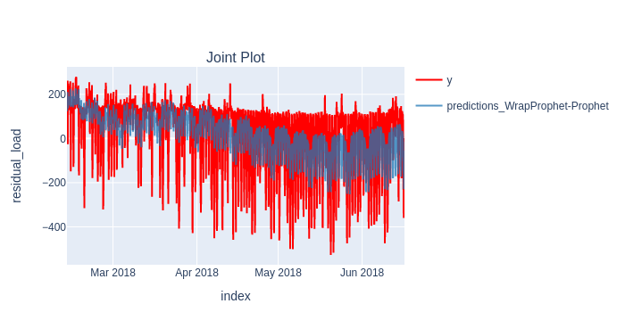
scorecard, predictions, trained_pipeline = train_evaluate(prophet, None, y, splitter, backend=BackendType.ray, krisi_args={"model_name":"prophet"})
4. Evaluating the results
                                               prophet
                     Mean Absolute Error  9.507563e+01
          Mean Absolute Percentage Error  7.955506e+13
Symmetric Mean Absolute Percentage Error  5.092002e-01
                      Mean Squared Error  1.477914e+04
                 Root Mean Squared Error  1.215695e+02
                               R-squared  4.268419e-01
                   Mean of the Residuals  6.361641e+00
     Standard Deviation of the Residuals  1.214232e+02
Finally, let's save the scorecard into a list, so we can compare the results later.
Using an Ensemble (Composite) model
Here we will build an Ensemble model that leverages the output of multiple models.

1. Model Building with fold-wrappers
We are going to define three different pipelines, each leveraging a different model and different features.
We can leverage the most popular modelling libraries, like StatsForecast, Sktime, XGBoost, etc. (the list can be found here).
Let's train a MSTL model that's implemented in StatsForecast, that can capture multiple seasonalities, with the WrapStatsForecast class from fold-wrappers. This is not strictly necessary, though, as the automatic wrapping also works for StatsForecast instaces as well.
from statsforecast.models import MSTL
from fold.models.wrappers import WrapStatsForecast, WrapStatsModels

mstl = WrapStatsForecast.from_model(MSTL([24, 168]))
2. Ensembling with fold
Finally, let's ensemble the two pipelines.
3. Training all pipelines seperately and within an ensemble
We'll use the same ExpandingWindowSplitter we have defined above, to make performance comparable.
from fold import train_evaluate

for name, pipeline in [
    ("mstl", mstl),
    ("univariate_ensemble",univariate_ensemble)
]:
    scorecard, predictions, pipeline_trained = train_evaluate(pipeline, None, y, splitter, krisi_args={"model_name":name})
    results.append((scorecard, predictions))
| rmse | mse | |
|---|---|---|
| prophet | 121.569502 | 14779.143772 |
| mstl | 118.703683 | 14090.564243 |
| univariate_ensemble | 105.962271 | 11228.002822 |
We see that our Ensemble model has beaten all individual models' performance - which is very usual in the time series context.
Using a single-step ahead forecaster (a baseline)
So far we've used models that were costly to update (or re-train) every day, therefore we were limited to training once for every week, then predicting the next week's target.
What if we could use a lightweight, "online" model, that can be updated on every timestamp?
And.. what if we just repeat the last value?
That'd be the Naive model you can load from fold.models.
from fold import train_evaluate
from fold.models import Naive

scorecard, predictions, trained_pipeline = train_evaluate(Naive(), None, y, splitter, krisi_args={"model_name":"naive"})
results.append((scorecard, predictions))
scorecard.print("minimal")
  0%|          | 0/18 [00:00<?, ?it/s]


  0%|          | 0/18 [00:00<?, ?it/s]
                                                 naive
                     Mean Absolute Error  3.911054e+01
          Mean Absolute Percentage Error  2.122351e+14
Symmetric Mean Absolute Percentage Error  2.038015e-01
                      Mean Squared Error  4.012944e+03
                 Root Mean Squared Error  6.334780e+01
                               R-squared  8.443718e-01
                   Mean of the Residuals -4.387701e-02
     Standard Deviation of the Residuals  6.335837e+01
We call this Adaptive Backtesting.
It looks like having access to last value really makes a difference: the baseline model beats all long-term forecasting models by a large margin.
It's extremely important to define our forecasting task well: 1. We need to think about what time horizon can and should forecast 2. And how frequently can we update our models.
Long-horizon (in this case, a week ahead) forecasts can be very unreliable, on the other hand, frequent, short-term forecasts are where Machine Learning shines (as we'll see in the next section).
Using exogenous variables with Tabular Models
So far we have been training univariate models, and ignored all the additional, exogenous variables that come with our data.
Let's try whether using this data boost our model's performance!
Building Models separately
We'll be using scikit-learn's HistGradientBoostingRegressor, their competing implementation of Gradient Boosted Trees. You don't need to wrap scikit-learn models or transformations when using it in fold, just pass it in directly to any pipeline.
from sklearn.ensemble import HistGradientBoostingRegressor

tree_model = HistGradientBoostingRegressor(max_depth=10)
Let's add both holiday and date-time features to our previous ensemble pipeline.
The data was gathered in the Region of Hessen, Germany -- so we pass in DE (we can pass in multiple regions). This transformation adds another column for holidays to our exogenous (X) features.
We're also adding the current hour, and day of week as integers to our exogenous features. This is one of the ways for our tabular model to capture seasonality.
from fold.transformations import AddHolidayFeatures, AddDateTimeFeatures

datetime = AddDateTimeFeatures(['hour', 'day_of_week', 'day_of_year'])
holidays = AddHolidayFeatures(['DE'])
Let's add a couple of lagged, exogenous values for our model. AddLagsX receives a tuple of column name and integer or list of lags, for each of which it will create a column in X.
We can easily create transformations of existing features on a rolling window basis with AddWindowFeatures as well, in this case, the last day's average value for all of our exogenous features.
We can "tie in" two separate pipelines with Concat, which concatenates all columns from all sources.
from fold.transformations import AddWindowFeatures, AddLagsX
from fold.composites import Concat

tree = [
    Concat([
        AddLagsX(("all",range(1,3))),
        AddWindowFeatures([("all", 24, "mean")]),
    ]),
    datetime,
    holidays,
    tree_model
]
Let's see how this performs!
We can also use fold's train, backtest to decouple these functionalities.
from fold import train, backtest

trained_pipeline = train(tree, X, y, splitter)
predictions = backtest(trained_pipeline, X, y, splitter)
scorecard = score(y[predictions.index], predictions.squeeze(), model_name="tabular_tree")

results.append((scorecard, predictions))
scorecard.print("minimal")
  0%|          | 0/18 [00:00<?, ?it/s]


  0%|          | 0/18 [00:00<?, ?it/s]
                                          tabular_tree
                     Mean Absolute Error  2.965292e+01
          Mean Absolute Percentage Error  2.123209e+14
Symmetric Mean Absolute Percentage Error  1.591514e-01
                      Mean Squared Error  2.637592e+03
                 Root Mean Squared Error  5.135749e+01
                               R-squared  8.977101e-01
                   Mean of the Residuals -1.747140e+00
     Standard Deviation of the Residuals  5.133635e+01
Creating an Ensemble of Tabular models
First let's creat two more models: * an Sklearn LinearRegressor * and an XGBoostRegressor instance
We are also going to use the HistGradientBoostingRegressor pipeline that we defined prior.
from sklearn.linear_model import LinearRegression

lregression = [
    AddLagsX(('all',range(1,3))),
    datetime,
    LinearRegression()
]
from xgboost import XGBRegressor
from fold.models.wrappers.gbd import WrapXGB

xgboost = [
    AddLagsX(('all',range(1,3))),
    datetime,
    WrapXGB.from_model(XGBRegressor())
]
scorecard, predictions, pipeline_trained = train_evaluate(tabular_ensemble, X, y, splitter, krisi_args={"model_name":"tabular_ensemble"})
results.append((scorecard, predictions))
  0%|          | 0/18 [00:00<?, ?it/s]


  0%|          | 0/18 [00:00<?, ?it/s]
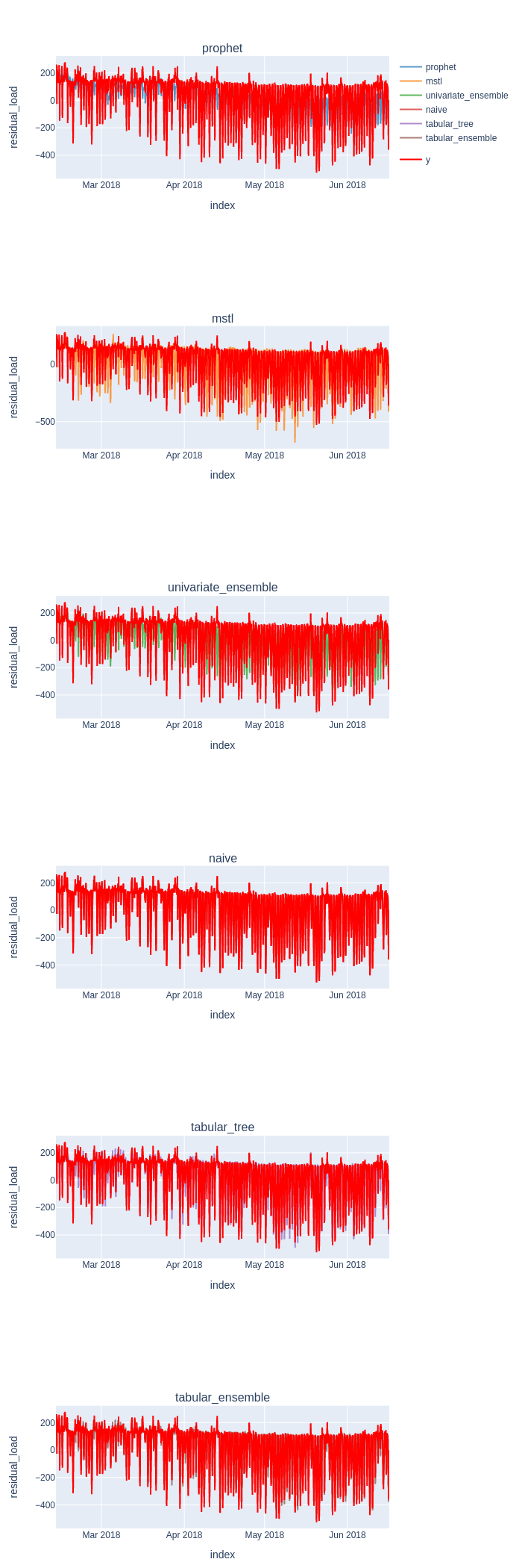
Comparing & Vizualising the results
| rmse | mae | mape | smape | mse | r_two | residuals_mean | residuals_std | |
|---|---|---|---|---|---|---|---|---|
| prophet | 121.569502 | 95.075627 | 7.955506e+13 | 0.509200 | 14779.143772 | 0.426842 | 6.361641 | 121.423231 |
| mstl | 118.703683 | 68.464305 | 1.846641e+14 | 0.279174 | 14090.564243 | 0.453546 | 13.258315 | 117.980649 |
| univariate_ensemble | 105.962271 | 73.283533 | 1.321096e+14 | 0.356740 | 11228.002822 | 0.564561 | 9.809978 | 105.524826 |
| naive | 63.347800 | 39.110541 | 2.122351e+14 | 0.203802 | 4012.943794 | 0.844372 | -0.043877 | 63.358374 |
| tabular_tree | 51.357493 | 29.652915 | 2.123209e+14 | 0.159151 | 2637.592134 | 0.897710 | -1.747140 | 51.336346 |
| tabular_ensemble | 48.228591 | 28.165175 | 2.113763e+14 | 0.153255 | 2325.997006 | 0.909794 | -2.690336 | 48.161544 |
In this simplistic, unfair comparison, it looks like the tabular models (and the Naive baseline) that have access to the previous value (and the exogenous variables) outperform the univariate models that are only re-trained every week.
We can't really draw general conclusions from this work, though.
Unlike NLP and Computer vision, Time Series data is very heterogeneous, and a Machine Learning approach that works well for one series may be an inferior choice for your specific usecase.
But now we have an easy way to compare the different pipelines, with unprecedented speed, by using a unified interface, with fold.
all_predictions =[predictions.squeeze().rename(scorecard.metadata.model_name) for scorecard, predictions in results]

plot_y_predictions(y[predictions.index], all_predictions, y_name="residual_load", mode='seperate')
Want to know more? Visit fold's Examples page, and access all the necessary snippets you need for you to build a Time Series ML pipeline!