Benchmarking the speed of fold and SKTime.

Installing libraries, defining utility functions

%%capture
pip install --quiet fold-core fold-models krisi fold-wrappers matplotlib seaborn xgboost plotly prophet statsforecast statsmodels ray kaleido sktime pmdarima

from time import monotonic
import pandas as pd
from collections import defaultdict
from krisi import score
from krisi.report import plot_y_predictions
import plotly.io as pio
pio.renderers.default = "png"

class Timing:
    results = defaultdict(lambda: defaultdict(dict))

    def record_time(self, model_name: str, framework: str):
        def wrapper( function, *args, **kwargs):
            start_time = monotonic()
            return_value = function(*args, **kwargs)
            print(f"Run time: {monotonic() - start_time} seconds")

            self.results[framework][model_name] = monotonic() - start_time
            return return_value
        return wrapper
    def summary(self):
        pd.set_option('display.max_rows', None)
        pd.set_option('display.max_columns', None)
        pd.set_option('display.colheader_justify', 'center')
        pd.set_option('display.precision', 3)
        display(pd.DataFrame(self.results))

timing = Timing()

def flatten_result_windows(series: pd.Series) -> pd.Series:
    return pd.concat(series.to_list())

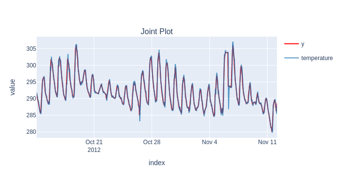
Data Loading

from fold.utils.dataset import get_preprocessed_dataset

X, y = get_preprocessed_dataset(
    "weather/historical_hourly_la", target_col="temperature", resample="H", shorten=1000
)

print(X.head());
print(y.head());
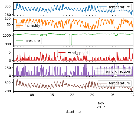
pd.concat([y,X], axis='columns').plot(subplots=True);

                     humidity  pressure  wind_speed  wind_direction  \
datetime                                                              
2012-10-01 13:00:00      88.0    1013.0         0.0             0.0   
2012-10-01 14:00:00      88.0    1013.0         0.0             0.0   
2012-10-01 15:00:00      88.0    1013.0         0.0             0.0   
2012-10-01 16:00:00      88.0    1013.0         0.0             0.0   
2012-10-01 17:00:00      88.0    1013.0         0.0             0.0

                     temperature  
datetime                          
2012-10-01 13:00:00   291.870000  
2012-10-01 14:00:00   291.868186  
2012-10-01 15:00:00   291.862844  
2012-10-01 16:00:00   291.857503  
2012-10-01 17:00:00   291.852162  
datetime
2012-10-01 13:00:00    291.868186
2012-10-01 14:00:00    291.862844
2012-10-01 15:00:00    291.857503
2012-10-01 16:00:00    291.852162
2012-10-01 17:00:00    291.846821
Freq: H, Name: temperature, dtype: float64

# Default values that both sktime and fold will receive

step_size = 50
initial_train_size = 300
lag_length_for_tabular_models = 10
fh=list(range(1, step_size+1))

SKTime - Long forecasting horizon (Time Series Cross-Validation)

from sktime.forecasting.model_evaluation import evaluate
from sktime.forecasting.model_selection import ExpandingWindowSplitter as SKTimeExpandingWindowSplitter
from sktime.forecasting.naive import NaiveForecaster
from sktime.forecasting.arima import ARIMA
from sktime.pipeline import make_pipeline
from sktime.forecasting.compose import make_reduction

cv = SKTimeExpandingWindowSplitter(initial_window=initial_train_size, step_length=step_size, fh=fh)

Naive

forecaster = NaiveForecaster(strategy="last")
results = timing.record_time('naive', 'sktime (long-fh)')(evaluate, forecaster=forecaster, y=y, X=X, cv=cv, return_data=True, error_score='raise')
predictions = flatten_result_windows(results['y_pred']).rename("naive")
plot_y_predictions(y[predictions.index], predictions.to_frame(), mode="overlap")
score(y[predictions.index], predictions)[['rmse']].print('minimal')

Run time: 0.32869669699999804 seconds

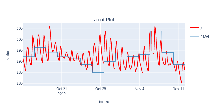
                                            naive
                 Root Mean Squared Error  5.36894

Statsmodels ARIMA

forecaster = ARIMA((1,1,0))

results = timing.record_time('arima', 'sktime (long-fh)')(evaluate, forecaster=forecaster, y=y, cv=cv, return_data=True, error_score='raise')
predictions = flatten_result_windows(results['y_pred'])
plot_y_predictions(y[predictions.index], predictions.to_frame(), mode="overlap")
score(y[predictions.index], predictions)[['rmse']].print('minimal')

Run time: 2.449221571999999 seconds

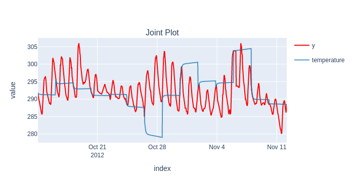
                                          temperature
                 Root Mean Squared Error     6.743475

A seasonal ARIMA - not suprisingly - provides much better results, but because of the slowness (and out of memory errors), we couldn't benchmark Statsmodels' implementation.

XGBoost

from xgboost import XGBRegressor
regressor = XGBRegressor(random_state=42)

forecaster = make_reduction(regressor, strategy="recursive", window_length=lag_length_for_tabular_models)
results = timing.record_time('xgboost', 'sktime (long-fh)')(evaluate, forecaster=forecaster, y=y, X=X, cv=cv, backend="multiprocessing", return_data=True, error_score='raise')
predictions = flatten_result_windows(results['y_pred'])
plot_y_predictions(y[predictions.index], predictions.to_frame(), mode="overlap")
score(y[predictions.index], predictions)[['rmse']].print('minimal')

Run time: 44.59098899100002 seconds

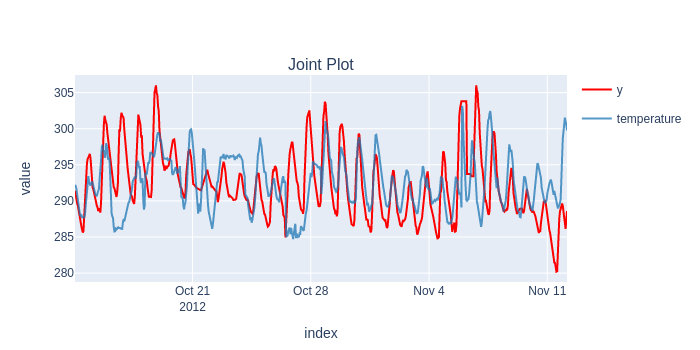
                                          temperature
                 Root Mean Squared Error     5.044424

Results

timing.summary()

	sktime (long-fh)
arima	2.449
naive	0.329
xgboost	44.591

SKTime may look fast on its own, but it definitely falls short when it comes to the real usefulness of Time Series Cross-Validation.

The models are static, stuck in the past between end of the training windows, they don't have access to the latest value, and therefore their predictions are way off.

Fold - Short forecasting horizon (Continuous Validation)

fold has the ability to update models within the test window, in an "online" manner:

from fold import train_evaluate, ExpandingWindowSplitter, BackendType
from fold.transformations import AddLagsX
from fold.models.wrappers import WrapXGB, WrapStatsModels
from fold.models import Naive
from statsmodels.tsa.arima.model import ARIMA as StatsModelARIMA
import ray
ray.init(ignore_reinit_error=True)

2023-04-17 11:07:04,950 INFO worker.py:1553 -- Started a local Ray instance.

Ray

Python version:	3.9.16
Ray version:	2.3.1

splitter = ExpandingWindowSplitter(initial_train_window=initial_train_size, step=step_size)

Naive

model = Naive()

scorecard, predictions, _ = timing.record_time('naive', 'fold (online)')(train_evaluate, model, None, y, splitter, backend=BackendType.no, silent=True)
plot_y_predictions(y[predictions.index], predictions, mode="overlap")
scorecard[['rmse']].print('minimal')

Run time: 0.17832120899998927 seconds

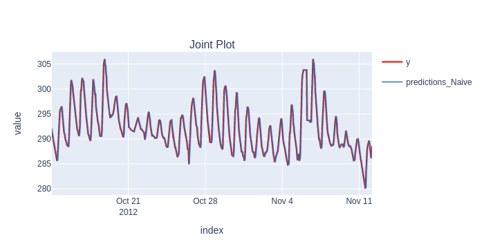
                                          predictions_Naive
                 Root Mean Squared Error        1.224

Statsmodels ARIMA (Online)

model = WrapStatsModels(StatsModelARIMA, init_args=dict(order=(1, 1, 0)), online_mode=True)
scorecard, predictions, _ = timing.record_time('arima', 'fold (online)')(train_evaluate, model, None, y, splitter, backend=BackendType.no, silent=True)
plot_y_predictions(y[predictions.index], predictions, mode="overlap")
scorecard[['rmse']].print('minimal')

Run time: 41.32513004100002 seconds

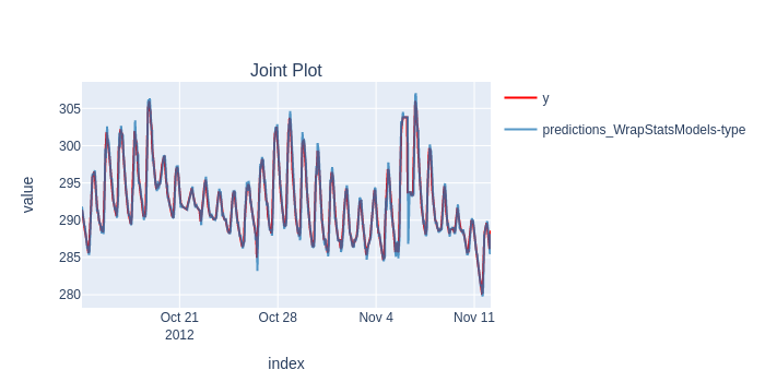
                                          predictions_WrapStatsModels-type
                 Root Mean Squared Error                0.927

XGBoost

from xgboost import XGBRegressor
model = XGBRegressor(random_state=42)
pipeline = [AddLagsX(("all", list(range(lag_length_for_tabular_models))) ), model]

scorecard, predictions, _ = timing.record_time('xgboost', 'fold (online)')(train_evaluate, pipeline, X, y, splitter, backend=BackendType.ray, silent=True)
plot_y_predictions(y[predictions.index], predictions, mode="overlap")
scorecard[['rmse']].print('minimal')

This results in much more realistic simulation of past performance (in case the last value is available in production).

Results

timing.summary()

	sktime (long-fh)	fold (online)
naive	0.329	0.180
arima	2.449	41.325
xgboost	44.591	13.256

And it's also substantially faster, except in the case of Statsmodels' ARIMA, which fold needs to update on every timestamp. Our own ARIMA (coming in April) will provide a ca. 100x speedup here.

SKTime - Short forecasting horizon (Continuous Validation)

cv = SKTimeExpandingWindowSplitter(initial_window=initial_train_size, step_length=1, fh=1)

Now let's see what SKTime's training speed would be like if we wanted to replicate "Continuous Validation", and the models having access to the latest value within the folds.

This means we'll need to update (not possible with the tested models) or fit a new model for every timestamp we return.

Naive

forecaster = NaiveForecaster(strategy="last")
results = timing.record_time('naive', 'sktime (online)')(evaluate, forecaster=forecaster, y=y, X=X, cv=cv, return_data=True, strategy="refit", error_score='raise')
predictions = flatten_result_windows(results['y_pred']).rename("naive")
plot_y_predictions(y[predictions.index], predictions.to_frame(), mode="overlap")
score(y[predictions.index], predictions)[['rmse']].print('minimal')

Run time: 18.046849753999993 seconds

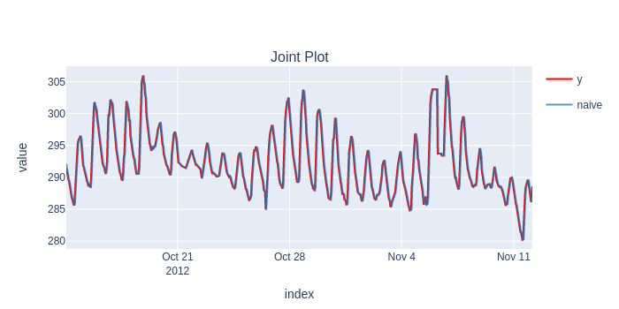
                                          naive
                 Root Mean Squared Error  1.224

Statsmodels ARIMA

from sktime.forecasting.arima import ARIMA
forecaster = ARIMA((1,1,0))

results = timing.record_time('arima', 'sktime (online)')(evaluate, forecaster=forecaster, y=y, cv=cv, return_data=True, error_score='raise')
predictions = flatten_result_windows(results['y_pred'])
plot_y_predictions(y[predictions.index], predictions.to_frame(), mode="overlap")
score(y[predictions.index], predictions)[['rmse']].print('minimal')

/usr/local/lib/python3.9/dist-packages/statsmodels/base/model.py:604: ConvergenceWarning:

Maximum Likelihood optimization failed to converge. Check mle_retvals



Run time: 106.65218957599996 seconds

                                          temperature
                 Root Mean Squared Error     0.927

XGBoost

from xgboost import XGBRegressor
regressor = XGBRegressor(random_state=42)

forecaster = make_reduction(regressor, strategy="recursive", window_length=lag_length_for_tabular_models)
results = timing.record_time('xgboost', 'sktime (online)')(evaluate, forecaster=forecaster, y=y, X=X, cv=cv, backend=None, return_data=True, error_score='raise')
predictions = flatten_result_windows(results['y_pred'])
plot_y_predictions(y[predictions.index], predictions.to_frame(), mode="overlap")
score(y[predictions.index], predictions)[['rmse']].print('minimal')

Run time: 759.161927353 seconds

                                          temperature
                 Root Mean Squared Error     1.018

Overall Results

timing.summary()

	sktime (long-fh)	fold (online)	sktime (online)
naive	0.329	0.180	18.048
arima	2.449	41.325	106.653
xgboost	44.591	13.256	759.163

Overall, fold provides a speedup between 3x and 100x, already.

When it comes to practice, we argue that this makes Continuos Validation feasible, compared to other tools out there.